SIR Model Basics Summary

Now that you have simulated the spread of an infectious disease in a population, let’s summarize some key takeaways.
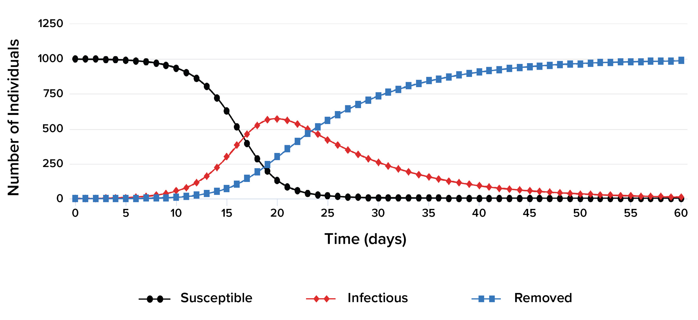
Example SIR Graph

The figure shows an example of an SIR graph. Your own SIR graph may look different depending on various factors, like the transmission and recovery probabilities you chose.

An example S-I-R graph. The x-axis measures Time in days and the y-axis measures number of individuals. A legend indicates that a black curve with circles graphs Susceptible individuals, a red curve with diamonds graphs Infectious individuals, and a blue curve with squares graphs Removed individuals.
An example SIR graph.

In general:

  • An SIR graph shows the number of individuals in three groups (susceptible, infectious, and removed) over time.
  • The graph shows time (e.g., days) on the x-axis and number of individuals on the y-axis.
  • Each curve (line) represents one group.
  • As individuals move between groups, the number of individuals in each group changes continuously over time. (However, the total number of individuals in the population stays the same.)

Analyzing and Interpreting an SIR Graph

An outbreak can be divided into three stages: early outbreak, peak outbreak, and late outbreak. When analyzing an SIR graph, we can estimate the population’s makeup (proportion of each group) at each stage.

An example S-I-R graph with three outbreak stages.
The example S-I-R graph with the x-axis measuring Time in days and the y-axis measuring Number of Individuals. There are three outbreak stages indicated with brackets above the graph labeled early, peak, and late. Three circles below the graph point to peaks of the 3 graphed lines, aligned with the outbreak stages. The first circle points to the high peak of the black curve with circles under the early outbreak stage and is labeled as 90% susceptible, 10% infectious and 0% removed. The second circle points to the peak of the red curve with diamonds under the peak outbreak stage and is labeled as 15% susceptible, 70% infectious and 15% removed. The third circle points to the peak of the blue curve with squares under the late outbreak stage and is labeled as 10% susceptible, 10% infectious and 80% removed. Legend for the graphical icons and lines: the black icon and curve with black circles show how the number of susceptible individuals changes througout the outbreak. The red coughing icon and curve with red diamonds show how the number of infectious individuals changes throughout the outbreak. The blue icon with raised arms and curve with blue squares show how the number of removed individuals changes througout the outbreak.
This illustration shows an example SIR graph (top) and representative population makeups (bottom). Makeups are from timepoints in the three main outbreak stages: (1) early outbreak, (2) peak outbreak, and (3) late outbreak.

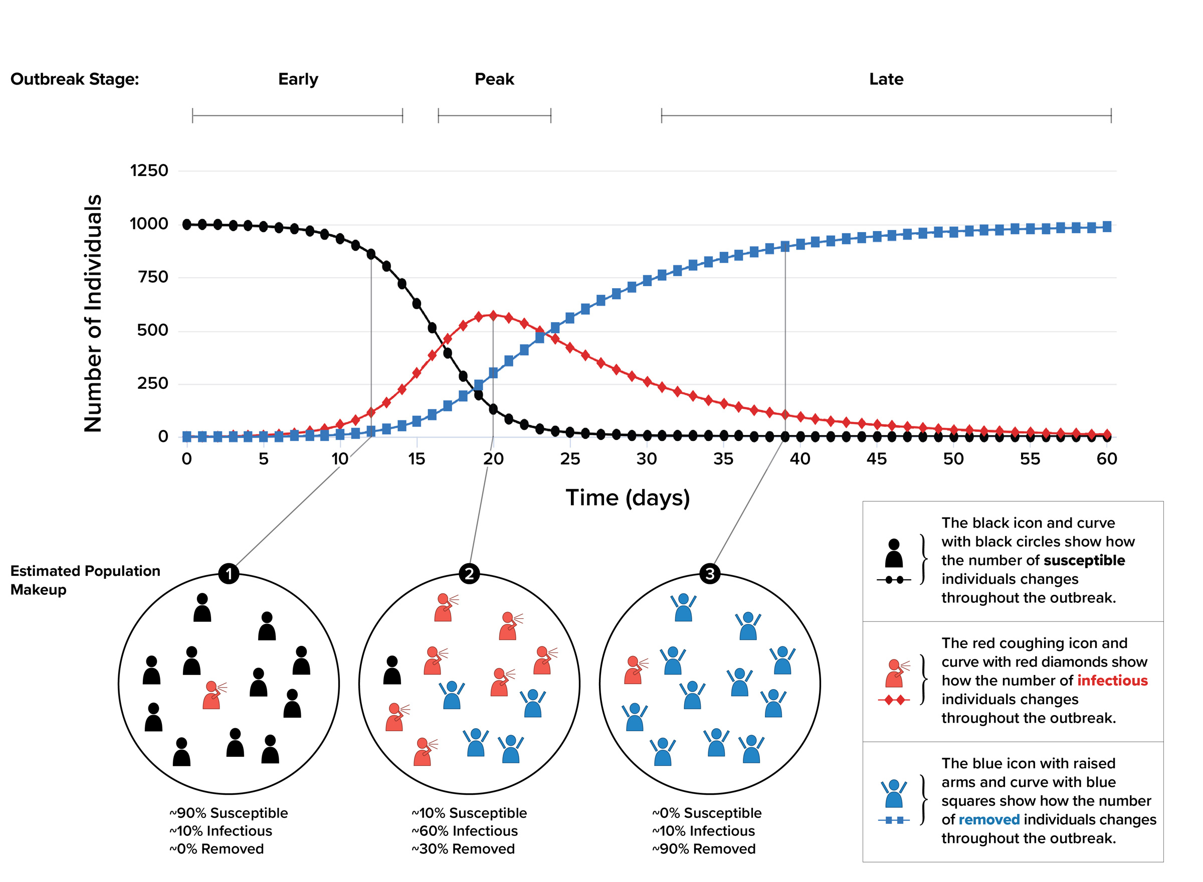
As you begin analyzing and interpreting your SIR graph, it is helpful to think about what is happening within each group at each stage in the outbreak.

Consider the shapes of the curves in each outbreak stage (early, peak, and late). What might these shapes indicate for each group?

The shapes of the curves depend on factors that affect how long an outbreak lasts and how many individuals are infected at any given time. As you experiment with the “Outbreak Simulator,” take note of how changing the transmission and recovery probabilities may change the shapes of the SIR curves.